2 - Reading an IDF file

As before, load the pyIBA library

# if pyIBA has been installed with pip3,
# the above 4 lines can be removed
import sys
from os.path import abspath
path_pyIBA = abspath('../../../..')
sys.path.insert(0, path_pyIBA)

# import pyIBA
from pyIBA import IDF

Loading the file

Example 1 - Creating a blank IDF demonstrated how to create an IDF file from raw data. Here we show how to edit/inspect an exiting IDF file. We use the file created previously:

file_path = '../Example1/idf_example1.xml'

and load it when creating the IDF object:

idf_file = IDF(file_path)

All the information included in the IDF object created on the previous example (1 - Creating a blank IDF) is now in the idf_file object.

The notes

Perhaps the first thing to read are the notes:

notes = idf_file.get_notes()

for note in notes:
    print(note)

print('Created by', idf_file.get_user())

This file was created during Example 1, it relates to a RBS measurement of a CoPt/SiO2 sample.
Something I did after the first note
Created by Miguel Sequeira

The beam parameters

To get the entire set of beam parameters, we can use the idf_file.get_geo_parameters():

idf_file.get_geo_parameters()

{'mode': 19,
 'window': [100, 1500],
 'projectile': '4He',
 'beam_energy': 2000.0,
 'beam_FWHM': 20.0,
 'geometry': 'IBM',
 'angles': ['30', '140'],
 'dect_solid': '11',
 'energy_calib': [2.28, 105.5],
 'charge': '5'}

Note that each of this parameters can be obtained individually. For instance, the beam energy and FWHM we can be retrieved using

energy, FWHM = idf_file.get_beam_energy()

print('Energy: %0.1f keV' %energy)
print('FWHM  : %0.1f keV' %FWHM)

Energy: 2000.0 keV
FWHM  : 20.0 keV

or, similarly, for the geometry of the experiment:

idf_file.get_geometry_type()

('IBM', ['30', '140'], None)

Please refer to help(idf_file.get_geo_parameters) to find all the individual methods

help(idf_file.get_geo_parameters)

Help on method get_geo_parameters in module pyIBA.main_idf:

get_geo_parameters(spectra_id=0) method of pyIBA.IDF.IDF instance
    Gets the entire set of parameters in a dictionary with the following format::

            params = {
                    'mode': 19,
                    'window': [100, 1500],
                    'projectile': 'He',
                    'beam_energy': 2000,
                    'beam_FWHM': 17,
                    'geometry': 'ibm',
                    'angles': [0, 160], # [incident, scattering]
                    'dect_solid': 7.2,
                    'energy_calib': [1, 0], # [m, b], E = m * channel + b,
                    'charge': 5
            }

    Each of these parameters can be obtained individually using the appropriate methods::

            params['window']= [self.get_window_min(), self.get_window_max()]
            params['projectile'] = self.get_beam_particles()
            params['beam_energy'], params['beam_FWHM'] = self.get_beam_energy()
            params['geometry'], params['angles'], _ = self.get_geometry_type()
            params['dect_solid'] = self.get_detector()
            params['energy_calib'] = self.get_energy_calibration()
            params['charge'] = self.get_charge()

    Args:
            spectra_id (int, optional): ID of the spectrum

    Returns:
            dictionary or None: Dictionary with the geometry parameters

    Raises:
            e: If data is missing

The spectrum

To get the spectrum from the file, you simple need to run:

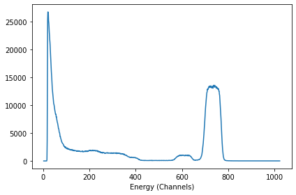
xx, yy = idf_file.get_dataxy()

Now, for instance if you want to print it using matplotlib:

#import matplotlib and increase the font size
import matplotlib.pyplot as plt
plt.rcParams.update({'font.size': 14})

#get the name of the file to use as label in the plot
name_file = idf_file.get_spectrum_file_name()

#create and plot the spectrum
plt.figure(figsize = (8,6))
plt.plot(xx, yy, label = name_file)

plt.xlabel('Channels')
plt.ylabel('Counts')
plt.legend();

The sample details

To get the elements in the sample, we run idf_file.get_elements() to get a dictionary similar to the one defined in Example 1 - Creating a blank IDF and used as input in idf_file.set_elements().

idf_file.get_elements()

{'nelements': 3,
 0: {'name': 'Co 1 Pt 1',
  'density': '',
  'concentration': ['0', '1'],
  'depth': ['0', '1000']},
 1: {'name': 'Si 1 O 2',
  'density': '',
  'concentration': ['0', '1'],
  'depth': ['0', '1000']},
 2: {'name': 'Si',
  'density': '',
  'concentration': ['0', '1'],
  'depth': ['300', '1e6']}}

Similarly, to obtain the depth profile of the sample, we use idf_file.get_profile() (see Example 1 - Creating a blank IDF):

idf_file.get_profile()

{'nlayers': 2,
 'names': ['Co 1 Pt 1', 'Si 1 O 2', 'Si'],
 0: {'thickness': '390', 'concentrations': ['100', '0', '0']},
 1: {'thickness': '550', 'concentrations': ['0', '100', '0']},
 2: {'thickness': '4000000', 'concentrations': ['0', '0', '100']}}

Quick check

If you want to print out the information on the file, in a text fashion (i.e. without possibility of changing the values), you can use print_idf_file() (see also Example 1 and Example A2).

idf_file.print_idf_file()

=============== idf_example1 ===============
../Example1/idf_example1.xml
Miguel Sequeira

------------------  Notes  ------------------
This file was created during Example 1, it relates to a RBS measurement of a CoPt/SiO2 sample.
Something I did after the first note

------------------ Elements -----------------
nelements        3

 - - - Element 0 - - -
name             Co 1 Pt 1
density
concentration    ['0', '1']
depth            ['0', '1000']

 - - - Element 1 - - -
name             Si 1 O 2
density
concentration    ['0', '1']
depth            ['0', '1000']

 - - - Element 2 - - -
name             Si
density
concentration    ['0', '1']
depth            ['300', '1e6']

------------------ Profile -----------------
nlayers                  2
names            ['Co 1 Pt 1', 'Si 1 O 2', 'Si']

 - - - Layer 0 - - -
thickness                390
concentrations           ['100', '0', '0']

 - - - Layer 1 - - -
thickness                550
concentrations           ['0', '100', '0']

 - - - Layer 2 - - -
thickness                4000000
concentrations           ['0', '0', '100']



-------- Spectrum 0 (RBS2PT50CO50_30.odf) --------
Technique       RBS


Projectile       4He
Beam energy      2000.0
Beam fwhm        20.0
Geometry         IBM
Angles           ['30', '140']
Dect solid       11
Energy calib     [2.28, 105.5]
Charge           5